Exploratory Data Analysis (EDA) and Data Preparation

Dataset:

• Loan Status Data for Credit Scoring
• Filename: loans_train.csv
• Target variable: Loan_Status

Import libraries

import numpy as np
import pandas as pd
import matplotlib.pyplot as plt
import seaborn as sns
sns.set_style("whitegrid")
sns.set_context("paper", font_scale=1.0) 

%matplotlib inline

# Set Options for display
pd.options.display.max_rows = 1000
pd.options.display.max_columns = 100
pd.options.display.float_format = '{:.2f}'.format

#Filter Warnings
import warnings
warnings.filterwarnings('ignore')

Load the dataset

• Specify the parameters (filepath, index column)
• Check for Date-Time Columns to Parse Dates
• Check Encoding if file does not load correctly

# to check your working directory
%pwd

# to change your working directory, use
# %cd

'C:\\Users\\cbaruc\\Downloads\\EDA'

df = pd.read_csv('loans_train.csv')

Describe the data

Verifying the data: Look out for the following

• Unexpected missing values
• Incorrect or unexpected data types and format
• Duplicates
• Unexpected dimesions (i.e. missing rows or columns)
• Incorrect spelling
• Mixed cases for strings
• Unexpected outliers or anomalous values
• Inconsistent or incorrect units of measurements

# Check for unexpected missing values
total = df.isnull().sum().sort_values(ascending=False)
total

Credit_History       50
Self_Employed        32
LoanAmount           22
Dependents           15
Loan_Amount_Term     14
Gender               13
Married               3
Loan_ID               0
Education             0
ApplicantIncome       0
CoapplicantIncome     0
Property_Area         0
Loan_Status           0
dtype: int64

# Check for Incorrect or unexpected data type & format
df.dtypes

Loan_ID               object
Gender                object
Married               object
Dependents            object
Education             object
Self_Employed         object
ApplicantIncome        int64
CoapplicantIncome    float64
LoanAmount           float64
Loan_Amount_Term     float64
Credit_History       float64
Property_Area         object
Loan_Status           object
dtype: object

# Check for duplicates
df.duplicated().value_counts()

False    614
Name: count, dtype: int64

# Data Preparation - Handle Duplicates
df.drop_duplicates(inplace=True)

# Check Categorical Column Values
df.select_dtypes(include=['object']).head()

	Loan_ID	Gender	Married	Dependents	Education	Self_Employed	Property_Area	Loan_Status
0	LP001002	Male	No	0	Graduate	No	Urban	Y
1	LP001003	Male	Yes	1	Graduate	No	Rural	N
2	LP001005	Male	Yes	0	Graduate	Yes	Urban	Y
3	LP001006	Male	Yes	0	Not Graduate	No	Urban	Y
4	LP001008	Male	No	0	Graduate	No	Urban	Y

# Check for misspellings and mixed cases for Categorical Data
df.select_dtypes(include=['object']).describe()

	Loan_ID	Gender	Married	Dependents	Education	Self_Employed	Property_Area	Loan_Status
count	614	601	611	599	614	582	614	614
unique	614	2	2	4	2	2	3	2
top	LP001002	Male	Yes	0	Graduate	No	Semiurban	Y
freq	1	489	398	345	480	500	233	422

# Handle date features if any
try:
    df['Year'] = df.Date.dt.year
    df['Month'] = df.Date.dt.month
    df['Day']=df.Date.dt.day
    df['Week'] = df.Date.dt.isocalendar().week

except:
    print("No date features")

No date features

Visualize & Analyze Univariate Numeric Variables

df_num = df.select_dtypes(include=['float64','int64'])
df_num.describe()

	ApplicantIncome	CoapplicantIncome	LoanAmount	Loan_Amount_Term	Credit_History
count	614.00	614.00	592.00	600.00	564.00
mean	5403.46	1621.25	146.41	342.00	0.84
std	6109.04	2926.25	85.59	65.12	0.36
min	150.00	0.00	9.00	12.00	0.00
25%	2877.50	0.00	100.00	360.00	1.00
50%	3812.50	1188.50	128.00	360.00	1.00
75%	5795.00	2297.25	168.00	360.00	1.00
max	81000.00	41667.00	700.00	480.00	1.00

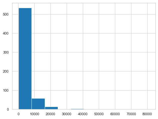
# Plot histograms, distplots, box plots, and/or density plots
df.ApplicantIncome.hist() # histograms

<Axes: >

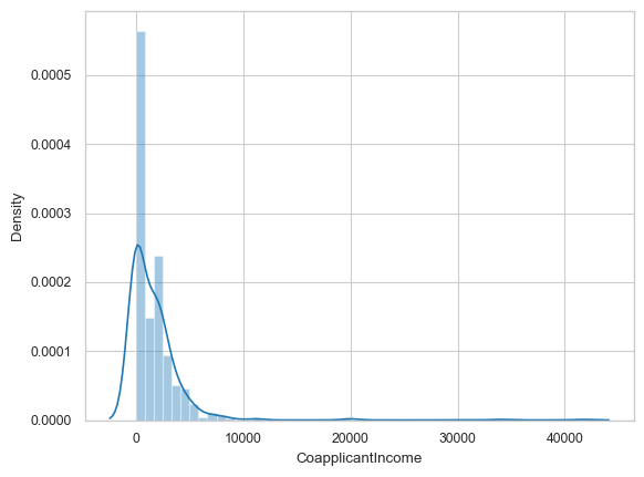
sns.distplot(df['CoapplicantIncome']) # distplots

<Axes: xlabel='CoapplicantIncome', ylabel='Density'>

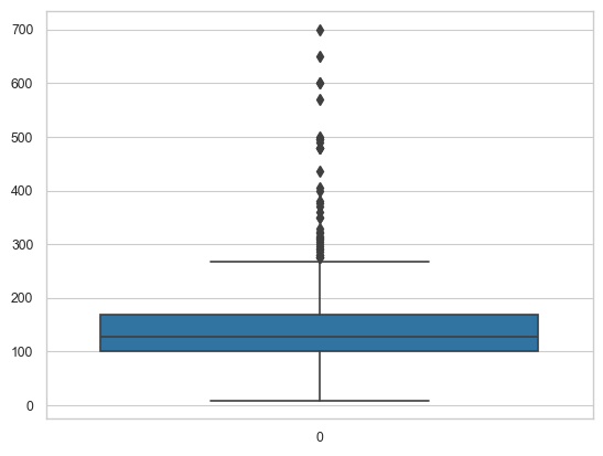
sns.boxplot(df['LoanAmount']) # boxplots

<Axes: >

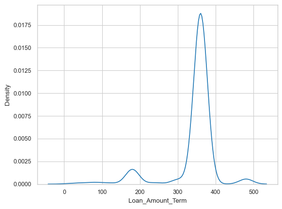
sns.kdeplot(df.Loan_Amount_Term) # density plot

<Axes: xlabel='Loan_Amount_Term', ylabel='Density'>

Data Preparation - Handle unexpected outliers

# Use the function to handle unexpected outliers

def remove_Outliers(df,col_name):
    print("Orig DF Size:"+ str(df.shape) )
    Q1 = np.quantile(df[col_name],0.25)

    Q3 = np.quantile(df[col_name],0.75)

    IQR = Q3 - Q1

    lower_limit = Q1 - (1.5*IQR)
    upper_limit = Q3 + (1.5*IQR)

    print("Lower fence: %.2f" % lower_limit)
    print("Upper fence: %.2f" % upper_limit)
    
    df_new = df[(df[col_name] > lower_limit) & (df[col_name] < upper_limit)]
    print("New DF Size:"+ str(df_new.shape) )
    return df_new

df.shape

(614, 13)

df_temp = remove_Outliers(df, 'ApplicantIncome')
df_temp.shape

Orig DF Size:(614, 13)
Lower fence: -1498.75
Upper fence: 10171.25
New DF Size:(564, 13)





(564, 13)

Visualize & Analyze Univariate Categorical Variables

df_cat = df_temp.select_dtypes(include=['object'])
df_cat.describe()

	Loan_ID	Gender	Married	Dependents	Education	Self_Employed	Property_Area	Loan_Status
count	564	554	561	550	564	534	564	564
unique	564	2	2	4	2	2	3	2
top	LP001002	Male	Yes	0	Graduate	No	Semiurban	Y
freq	1	451	364	321	432	467	215	389

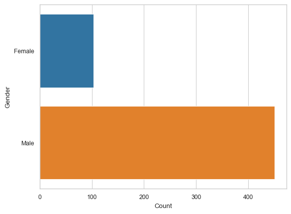
# Plot barplots, countplots
gender_counts = df_cat.groupby('Gender').size().reset_index(name='Count')
sns.barplot(x='Count', y='Gender', data=gender_counts) # barplots

<Axes: xlabel='Count', ylabel='Gender'>

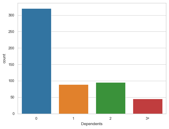
# Plot barplots, countplots
sns.countplot(x='Dependents', data = df_cat) # countplots

<Axes: xlabel='Dependents', ylabel='count'>

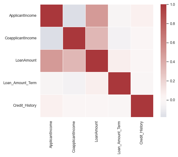
Run Multivariate analysis and plots

# Check correlation by computing and plotting correlation matrix
corrmat = df_temp.corr(numeric_only=True)
corrmat

	ApplicantIncome	CoapplicantIncome	LoanAmount	Loan_Amount_Term	Credit_History
ApplicantIncome	1.00	-0.18	0.49	-0.04	0.05
CoapplicantIncome	-0.18	1.00	0.34	-0.06	-0.00
LoanAmount	0.49	0.34	1.00	0.07	-0.01
Loan_Amount_Term	-0.04	-0.06	0.07	1.00	-0.02
Credit_History	0.05	-0.00	-0.01	-0.02	1.00

sns.heatmap(corrmat,  cmap="vlag", center = 0,  vmax=1, square=True, linewidths=.5)

<Axes: >

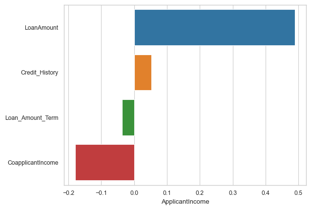
corr = corrmat.sort_values('ApplicantIncome', ascending=False)
sns.barplot(x = corr.ApplicantIncome[1:], y = corr.index[1:], orient='h')

<Axes: xlabel='ApplicantIncome'>

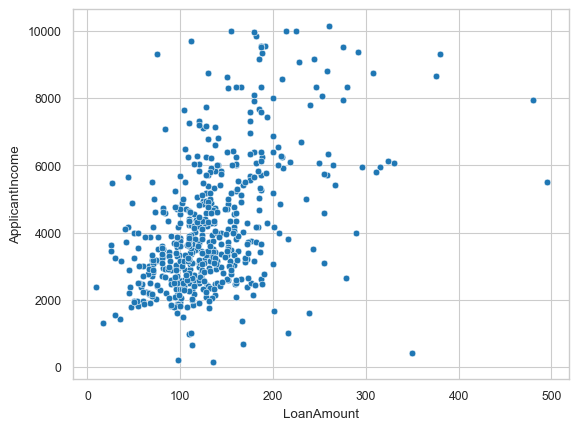
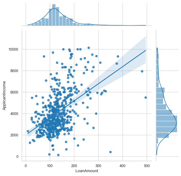
Plot Quantitative vs. Quantitative values together, any observations/insights?

# Plot scatterplots, jointplots, regplots, and pairplots if needed
sns.scatterplot(x='LoanAmount', y='ApplicantIncome', data = df_temp) # scatterplots

<Axes: xlabel='LoanAmount', ylabel='ApplicantIncome'>

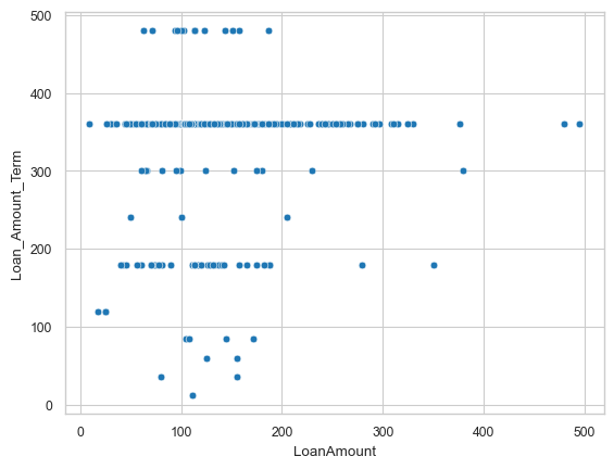
sns.scatterplot(x='LoanAmount', y='Loan_Amount_Term', data = df_temp) #scatterplots

<Axes: xlabel='LoanAmount', ylabel='Loan_Amount_Term'>

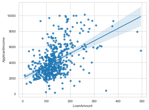
sns.regplot(x='LoanAmount', y='ApplicantIncome', data = df_temp) #regplots

<Axes: xlabel='LoanAmount', ylabel='ApplicantIncome'>

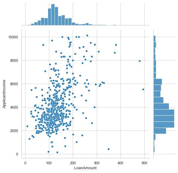
sns.jointplot(x='LoanAmount', y='ApplicantIncome', data = df_temp) #regplots

<seaborn.axisgrid.JointGrid at 0x1cfa8501910>

sns.jointplot(x='LoanAmount', y='ApplicantIncome', data=df_temp, kind='reg')

<seaborn.axisgrid.JointGrid at 0x1cfa9701e90>

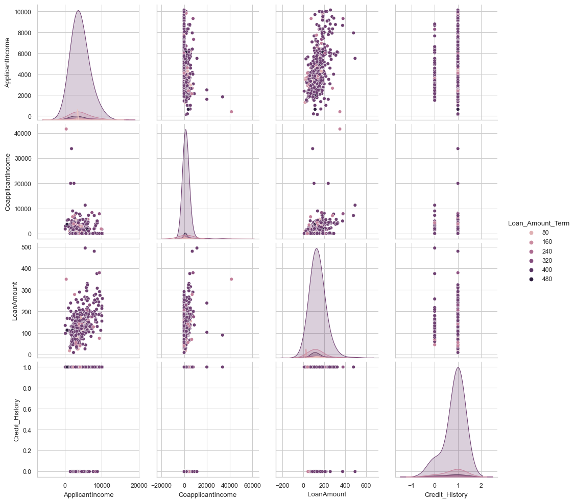
sns.pairplot(df_temp, hue='Loan_Amount_Term', diag_kws={'bw': 1})

<seaborn.axisgrid.PairGrid at 0x1cf9ac98f10>

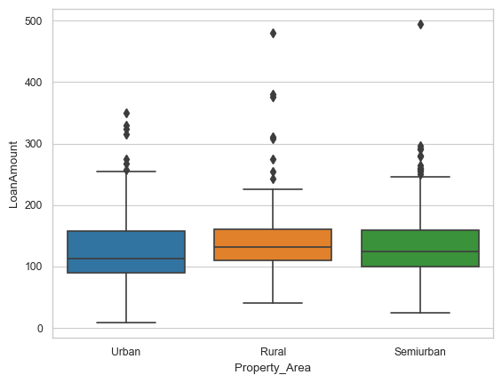
Plot Qualitative vs. Quantitative values together, any observations/insights?

# Plot boxplots, violin plots, catplots
sns.boxplot(data=df_temp,x="Property_Area", y="LoanAmount")

<Axes: xlabel='Property_Area', ylabel='LoanAmount'>

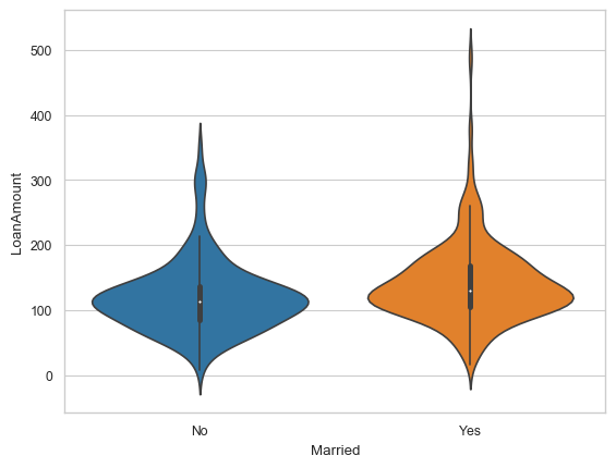
# Plot boxplots, violin plots, catplots
sns.violinplot(data=df_temp,x="Married", y="LoanAmount")

<Axes: xlabel='Married', ylabel='LoanAmount'>

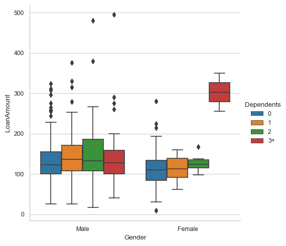
sns.catplot(data=df_temp,x="Gender", y="LoanAmount", hue = "Dependents", kind="box")

<seaborn.axisgrid.FacetGrid at 0x1cfb890c490>

Data Preparation - Category to Numeric

Convert any ordinal features to numeric

# Use OrdinalEncoder or substitution
from sklearn.preprocessing import LabelEncoder
from sklearn.preprocessing import OrdinalEncoder

le = LabelEncoder()
df_temp["Dependents_new"] = le.fit_transform(df_temp['Dependents'])

dep = df_temp.Dependents.value_counts().sort_values(ascending=False)
dep_new = df_temp.Dependents_new.value_counts().sort_values(ascending=False)
pd.DataFrame([dep.index.values,dep_new.index.values,dep.values], index=['dependents','dependents_new','values']).T

	dependents	dependents_new	values
0	0	0	321
1	2	2	95
2	1	1	89
3	3+	3	45
4	NaN	4.00	NaN

# Using substitution
df_temp['Property_Area_new'] = df_temp['Property_Area']
df_temp = df_temp.replace({'Property_Area_new':{'Urban':0,'Rural':1,'Semiurban':2}})

prop = df_temp.Property_Area.value_counts().sort_values(ascending=False)
prop_new = df_temp.Property_Area_new.value_counts().sort_values(ascending=False)
pd.DataFrame([prop.index.values,prop_new.index.values,prop.values], index=['prop_area','prop_area_new','values']).T

	prop_area	prop_area_new	values
0	Semiurban	2	215
1	Urban	0	181
2	Rural	1	168

df_temp.drop(['Dependents', 'Property_Area'],axis = 1, inplace = True)

df_temp.columns

Index(['Loan_ID', 'Gender', 'Married', 'Education', 'Self_Employed',
       'ApplicantIncome', 'CoapplicantIncome', 'LoanAmount',
       'Loan_Amount_Term', 'Credit_History', 'Loan_Status', 'Dependents_new',
       'Property_Area_new'],
      dtype='object')

Convert nominal features to numeric

df_temp.dtypes

Loan_ID               object
Gender                object
Married               object
Education             object
Self_Employed         object
ApplicantIncome        int64
CoapplicantIncome    float64
LoanAmount           float64
Loan_Amount_Term     float64
Credit_History       float64
Loan_Status           object
Dependents_new         int32
Property_Area_new      int64
dtype: object

# use pd.get_dummies, make sure to join with original dataset and/or drop columns not needed

df_categ = df_temp[['Gender', 'Married', 'Education', 'Self_Employed','Loan_Status']]
df_cat_dummies = pd.get_dummies(df_categ)
df_cat_dummies.head()

	Gender_Female	Gender_Male	Married_No	Married_Yes	Education_Graduate	Education_Not Graduate	Self_Employed_No	Self_Employed_Yes	Loan_Status_N	Loan_Status_Y
0	False	True	True	False	True	False	True	False	False	True
1	False	True	False	True	True	False	True	False	True	False
2	False	True	False	True	True	False	False	True	False	True
3	False	True	False	True	False	True	True	False	False	True
4	False	True	True	False	True	False	True	False	False	True

df = df_temp.join(df_cat_dummies)

df.head()

	Loan_ID	Gender	Married	Education	Self_Employed	ApplicantIncome	CoapplicantIncome	LoanAmount	Loan_Amount_Term	Credit_History	Loan_Status	Dependents_new	Property_Area_new	Gender_Female	Gender_Male	Married_No	Married_Yes	Education_Graduate	Education_Not Graduate	Self_Employed_No	Self_Employed_Yes	Loan_Status_N	Loan_Status_Y
0	LP001002	Male	No	Graduate	No	5849	0.00	NaN	360.00	1.00	Y	0	0	False	True	True	False	True	False	True	False	False	True
1	LP001003	Male	Yes	Graduate	No	4583	1508.00	128.00	360.00	1.00	N	1	1	False	True	False	True	True	False	True	False	True	False
2	LP001005	Male	Yes	Graduate	Yes	3000	0.00	66.00	360.00	1.00	Y	0	0	False	True	False	True	True	False	False	True	False	True
3	LP001006	Male	Yes	Not Graduate	No	2583	2358.00	120.00	360.00	1.00	Y	0	0	False	True	False	True	False	True	True	False	False	True
4	LP001008	Male	No	Graduate	No	6000	0.00	141.00	360.00	1.00	Y	0	0	False	True	True	False	True	False	True	False	False	True

#drop original columns
df.drop(columns = df_categ.columns, axis = 1, inplace = True)

df['Loan_ID'] = df['Loan_ID'].str.extract('(\d+)', expand=False).astype(float)

df.head()

	Loan_ID	ApplicantIncome	CoapplicantIncome	LoanAmount	Loan_Amount_Term	Credit_History	Dependents_new	Property_Area_new	Gender_Female	Gender_Male	Married_No	Married_Yes	Education_Graduate	Education_Not Graduate	Self_Employed_No	Self_Employed_Yes	Loan_Status_N	Loan_Status_Y
0	1002.00	5849	0.00	NaN	360.00	1.00	0	0	False	True	True	False	True	False	True	False	False	True
1	1003.00	4583	1508.00	128.00	360.00	1.00	1	1	False	True	False	True	True	False	True	False	True	False
2	1005.00	3000	0.00	66.00	360.00	1.00	0	0	False	True	False	True	True	False	False	True	False	True
3	1006.00	2583	2358.00	120.00	360.00	1.00	0	0	False	True	False	True	False	True	True	False	False	True
4	1008.00	6000	0.00	141.00	360.00	1.00	0	0	False	True	True	False	True	False	True	False	False	True

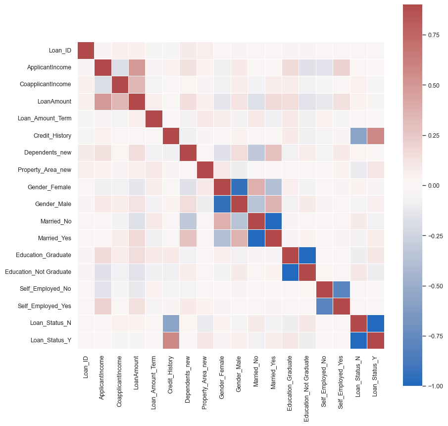
corrmat = df.corr()
plt.figure(figsize=(10,10))
sns.heatmap(corrmat,  cmap="vlag", center = 0,  vmax=.9, square=True, linewidths=.5)

<Axes: >

Scale the numeric columns excluding the target values

df.shape

(564, 18)

df.ApplicantIncome.describe()

count     564.00
mean     4124.72
std      1926.99
min       150.00
25%      2744.00
50%      3638.50
75%      5010.50
max     10139.00
Name: ApplicantIncome, dtype: float64

df.describe()

	Loan_ID	ApplicantIncome	CoapplicantIncome	LoanAmount	Loan_Amount_Term	Credit_History	Dependents_new	Property_Area_new
count	564.00	564.00	564.00	544.00	550.00	517.00	564.00	564.00
mean	1998.41	4124.72	1692.29	133.81	341.89	0.84	0.83	1.06
std	568.48	1926.99	2979.23	59.07	65.76	0.37	1.12	0.84
min	1002.00	150.00	0.00	9.00	12.00	0.00	0.00	0.00
25%	1539.50	2744.00	0.00	100.00	360.00	1.00	0.00	0.00
50%	1993.50	3638.50	1405.50	124.00	360.00	1.00	0.00	1.00
75%	2468.25	5010.50	2337.00	159.25	360.00	1.00	2.00	2.00
max	2990.00	10139.00	41667.00	495.00	480.00	1.00	4.00	2.00

# Separate the target variable(s)
df_x = df.drop(["Loan_Status_N","Loan_Status_Y"], axis=1)
y = df[["Loan_Status_N","Loan_Status_Y"]]    

# Perform scaling

#Import the MinMax Scaler
from sklearn.preprocessing import MinMaxScaler, StandardScaler, RobustScaler

#Instantiate the Scaler
scaler = MinMaxScaler()

#Fit to the data set
scaler.fit(df_x)

#Apply to the data set
scaled_data = scaler.transform(df_x)


#Optional:
#Convert to DataFrame for viewing
df_minmax = pd.DataFrame(scaled_data, columns=df_x.columns, index=df_x.index)

df_minmax.describe()

	Loan_ID	ApplicantIncome	CoapplicantIncome	LoanAmount	Loan_Amount_Term	Credit_History	Dependents_new	Property_Area_new	Gender_Female	Gender_Male	Married_No	Married_Yes	Education_Graduate	Education_Not Graduate	Self_Employed_No	Self_Employed_Yes
count	564.00	564.00	564.00	544.00	550.00	517.00	564.00	564.00	564.00	564.00	564.00	564.00	564.00	564.00	564.00	564.00
mean	0.50	0.40	0.04	0.26	0.70	0.84	0.21	0.53	0.18	0.80	0.35	0.65	0.77	0.23	0.83	0.12
std	0.29	0.19	0.07	0.12	0.14	0.37	0.28	0.42	0.39	0.40	0.48	0.48	0.42	0.42	0.38	0.32
min	0.00	0.00	0.00	0.00	0.00	0.00	0.00	0.00	0.00	0.00	0.00	0.00	0.00	0.00	0.00	0.00
25%	0.27	0.26	0.00	0.19	0.74	1.00	0.00	0.00	0.00	1.00	0.00	0.00	1.00	0.00	1.00	0.00
50%	0.50	0.35	0.03	0.24	0.74	1.00	0.00	0.50	0.00	1.00	0.00	1.00	1.00	0.00	1.00	0.00
75%	0.74	0.49	0.06	0.31	0.74	1.00	0.50	1.00	0.00	1.00	1.00	1.00	1.00	0.00	1.00	0.00
max	1.00	1.00	1.00	1.00	1.00	1.00	1.00	1.00	1.00	1.00	1.00	1.00	1.00	1.00	1.00	1.00

# Join back the target variables
df_prep = df_minmax.join(y)

df_prep.head()

	Loan_ID	ApplicantIncome	CoapplicantIncome	LoanAmount	Loan_Amount_Term	Credit_History	Dependents_new	Property_Area_new	Gender_Female	Gender_Male	Married_No	Married_Yes	Education_Graduate	Education_Not Graduate	Self_Employed_No	Self_Employed_Yes	Loan_Status_N	Loan_Status_Y
0	0.00	0.57	0.00	NaN	0.74	1.00	0.00	0.00	0.00	1.00	1.00	0.00	1.00	0.00	1.00	0.00	False	True
1	0.00	0.44	0.04	0.24	0.74	1.00	0.25	0.50	0.00	1.00	0.00	1.00	1.00	0.00	1.00	0.00	True	False
2	0.00	0.29	0.00	0.12	0.74	1.00	0.00	0.00	0.00	1.00	0.00	1.00	1.00	0.00	0.00	1.00	False	True
3	0.00	0.24	0.06	0.23	0.74	1.00	0.00	0.00	0.00	1.00	0.00	1.00	0.00	1.00	1.00	0.00	False	True
4	0.00	0.59	0.00	0.27	0.74	1.00	0.00	0.00	0.00	1.00	1.00	0.00	1.00	0.00	1.00	0.00	False	True

### Write the prepared dataset into a new file
#Save as a csv
df_prep.to_csv('\\Users\\cbaruc\\Downloads\\EDA\loans_train_prep.csv')